Skip to main content \(\newcommand{\N}{\mathbb N}
\newcommand{\Z}{\mathbb Z}
\newcommand{\Q}{\mathbb Q}
\newcommand{\R}{\mathbb R}
\newcommand{\lt}{<}
\newcommand{\gt}{>}
\newcommand{\amp}{&}
\definecolor{fillinmathshade}{gray}{0.9}
\newcommand{\fillinmath}[1]{\mathchoice{\colorbox{fillinmathshade}{$\displaystyle \phantom{\,#1\,}$}}{\colorbox{fillinmathshade}{$\textstyle \phantom{\,#1\,}$}}{\colorbox{fillinmathshade}{$\scriptstyle \phantom{\,#1\,}$}}{\colorbox{fillinmathshade}{$\scriptscriptstyle\phantom{\,#1\,}$}}}
\)
Section 25.4 Representations of Potential
Activity 25.4.1 . Warm-up.
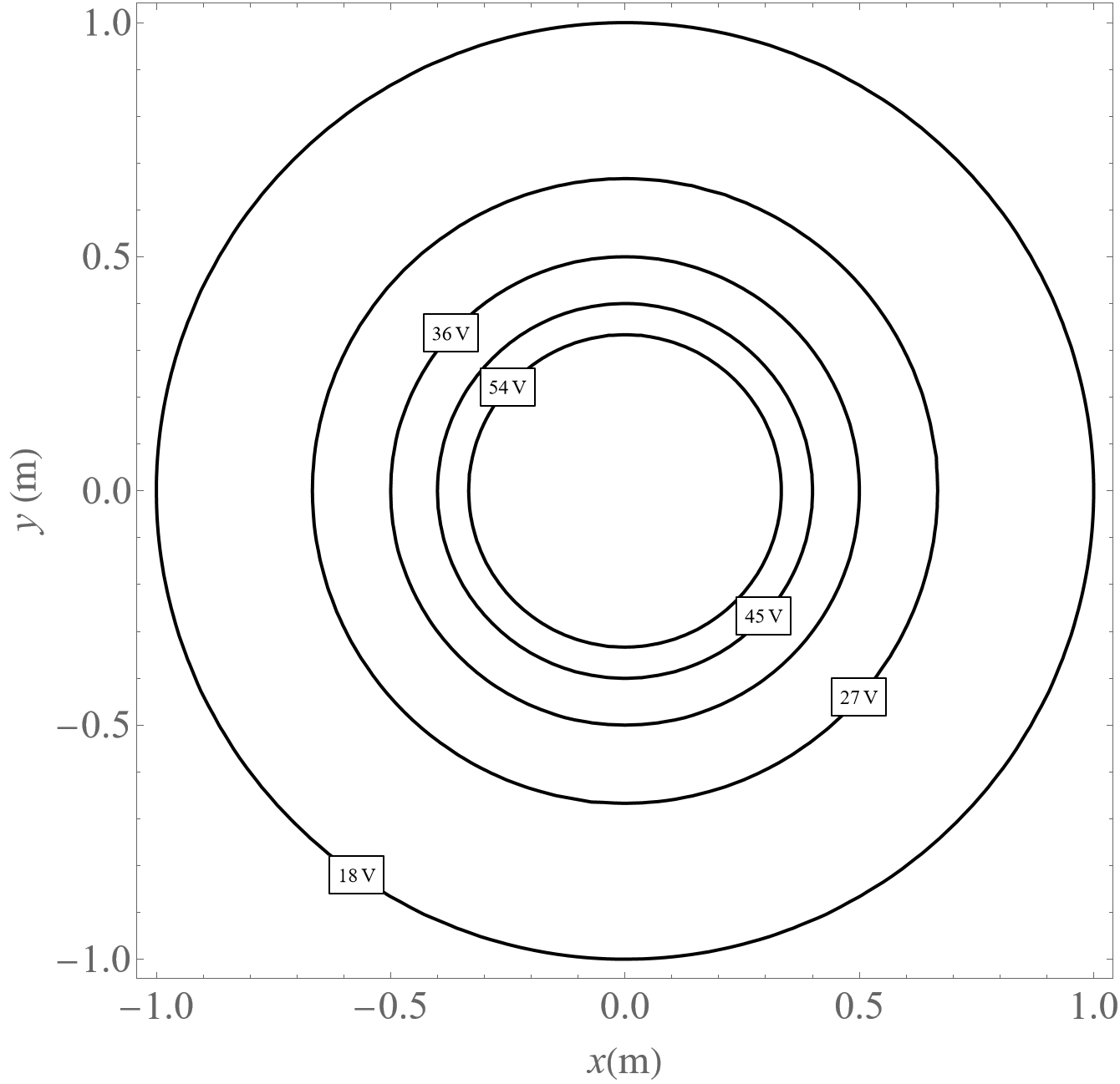
Consider the equipotentials below.
Figure 25.4.1. Equipotential lines.
(a) Draw a vector at each point to indicate the electric field.
(b) How can you tell the direction?
(c) Which point represents a larger
\(\vec{E}\text{?}\)
(d) Estimate the magnitude of
\(\vec{E}\) at each point.
Activity 25.4.2 . Potential for the Infinite Plate.
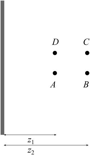
The electric field due to the infinite plate with charge density \(\sigma\) shown in the figure below has uniform magnitude and points perpendicular to the plate:
\begin{equation*}
\vec{E} = \frac{\sigma}{2\epsilon_0}\hat{z}
\end{equation*}
Figure 25.4.2. An infinitely large charged plate.
(a) Draw an electric field vector map.
(b) Use an integral to find
\(\Delta V\) between points A and B.
(c) Use an integral to find
\(\Delta V\) between points B and C.
(d) Draw equipotential lines (at least five!).
(e)
What happens to the potential if you travel the path:
\begin{equation*}
A \rightarrow B \rightarrow C \rightarrow D \rightarrow A
\end{equation*}
Activity 25.4.3 . Equipotentials.
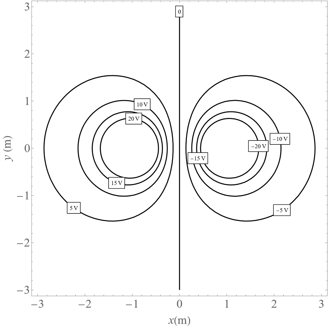
Now consider the equipotentials below
Figure 25.4.3. Equipotential lines.
(a) Rank the points by the value of the potential.
(b) Draw a vector at each point to indicate the electric field.
(c) Rank the points by the magnitude of the electric field.
(d)