Section 23.4 Gauss’s Law
Subsubsection Key Ideas
Principle 23.4.2. Gauss’s Law.
The net electric flux through any closed surface is proportional to the charge enclosed by that surface:
\begin{equation*}
\mathit{\Phi}_E = \frac{Q_{enc}}{\epsilon_0}
\end{equation*}
\begin{equation*}
\unicode{x222F}_{S} \vec{E}\cdot d\vec{A} = \frac{Q_{enc}}{\epsilon_0}
\end{equation*}
The closed circle on the integral symbol indicates that this is an integral over a closed surface. The symbol \(\epsilon_0\) is the Permittivity of Free Space and is related to the electrostatic constant \(k\text{.}\)
Gauss’s Law is extremely useful when your charge distribution has just the right symmetry. To effectively use Gauss’s Law, we need:
-
the electric field to be parallel to the area vector, \(d\vec{A}\)
-
the electric field to be uniform in magnitude along the surface
When the electric field and area vector are parallel, this will maximize, and simplify, the dot product in the integral. When the electric field is uniform along the surface, the magnitude of the electric field can then be pulled out of the integral since it no longer depends on where on the area of your surface you are looking. This is what makes Gauss’s Law powerful when calculating the magnitude of an electric field.
To use Gauss’s Law, you typically need to choose a “Gaussian surface” that adequately matches the symmetry of your charge distribution. Interestingly, the flux through a surface does not depend on the shape of the surface, because ultimately the flux through any surface is equal to \(\frac{Q_{enc}}{\epsilon_0}\text{,}\) but differently shaped surfaces will change, or potentially complicate, your calculations if you are directly calculating the flux through a surface.
Subsubsection Example Derivation: Point Charge
A straightforward application of Gauss’s Law is to confirm that the electric field created by a single point charge \(q\) located at the origin is
\begin{equation*}
\vec{E} = \frac{1}{4\pi\epsilon_o}\frac{q}{r^2}\hat{r}
\end{equation*}
Since the point charge is located the origin and the electric field points directly outward from the charge, the system exhibits spherical symmetry: that is, the electric field only depends on the distance \(r\text{.}\) As a result, a sphere of radius \(r\) is a natural choice for the Gaussian surface. The total charge enclosed by this surface is exactly \(q\text{,}\) so all that is left to calculate is the total flux. Writing the flux integral in spherical coordinates gives:
\begin{equation*}
\Phi_E = \unicode{x222F}_{S} \vec{E}\cdot d\vec{A} = \int_0^{2\pi}\int_0^\pi \left(E_r \hat{r}\right)\cdot \left(r^2\sin\theta d\theta d\phi \hat{r}\right)
\end{equation*}
Here \(E_r\) represents the magnitude of the electric field’s radial component (the other components of the electric field are zero). Resolving the dot product and then performing the integral gives:
\begin{equation*}
\Phi_E = \int_0^{2\pi}\int_0^\pi E_r r^2\sin\theta d\theta d\phi = 4\pi r^2 E_r
\end{equation*}
Last of all, relating this to the charge via Gauss’s Law results in the correct magnitude of the electric field!
\begin{equation*}
E_r = \frac{q}{4\pi\epsilon_0 r^2}
\end{equation*}
Subsubsection Activities
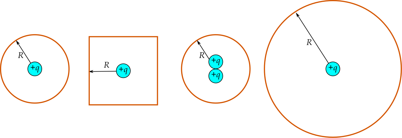
Explanation 23.4.1. Four Cases.
Rank the four cases below by the net electric flux through the shown Gaussian surface from greatest to least. Explain your reasoning.
Explanation 23.4.2. Straight Wire.
Suppose you have a straight wire with a uniform charge density, where the length of the wire is much, much greater than its width. What kind of Gaussian surface do you think you should choose for this charge distribution? Explain your reasoning.

