In general, quantities of motion like position and velocity are functions of time, in which case they might be written as \(\vec{r}(t)\) and \(\vec{v}(t)\text{.}\) When written in this way, it is often useful to graph position or velocity vs. time. Such a graph is known as a motion graph.
A motion graph is a graphical representation showing a motion quantity (like position or velocity) on the vertical axis and time on the horizontal axis.
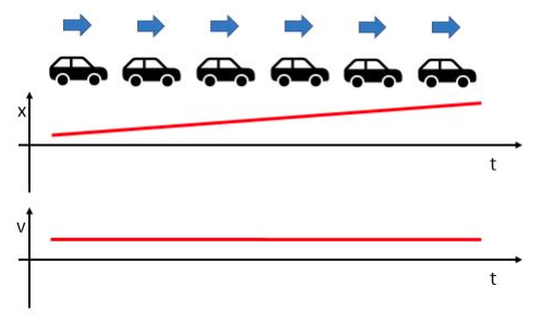
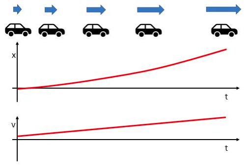
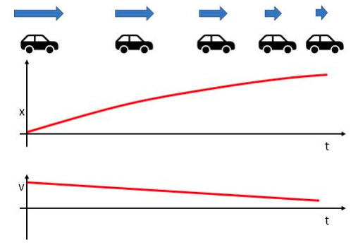
It is often useful to create motion graphs alongside motion diagrams to provide multiple ways of representing the same motion. There is a distinction between the two representations, however: the motion diagram has one image for each equal \(\Delta t\text{.}\) The position vs. time and velocity vs. time graphs also have equally spaced time increments, but unlike the strobe diagram, they are equally spaced along the axes. The two ways of visualizing motion are qualitatively correct, but you cannot make a direct vertical comparison.
You know that velocity and position are related by \(\vec{v} = \frac{d\vec{r}}{dt}\text{.}\) How does this relationship appear on graphs of velocity and position vs. time for the same object?
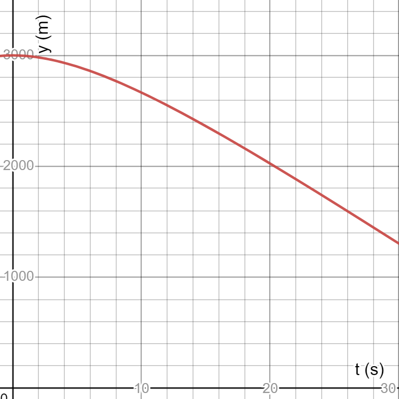
The graph of position vs. time below shows the location of a skydiver. Use the graph to create (1) a description in words of the skydiver’s motion, (2) a graph of the skydiver’s velocity vs. time, and (3) a motion diagram for the skydiver. Include an estimate of the skydiver’s speed at \(t = 26\) s.