You now have two major representations for describing motion: Motion Diagram and Motion Graph. Coordinating these representations with words and equations can give you a powerful understanding of an object’s motion.
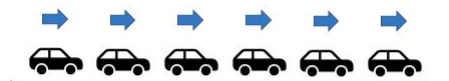
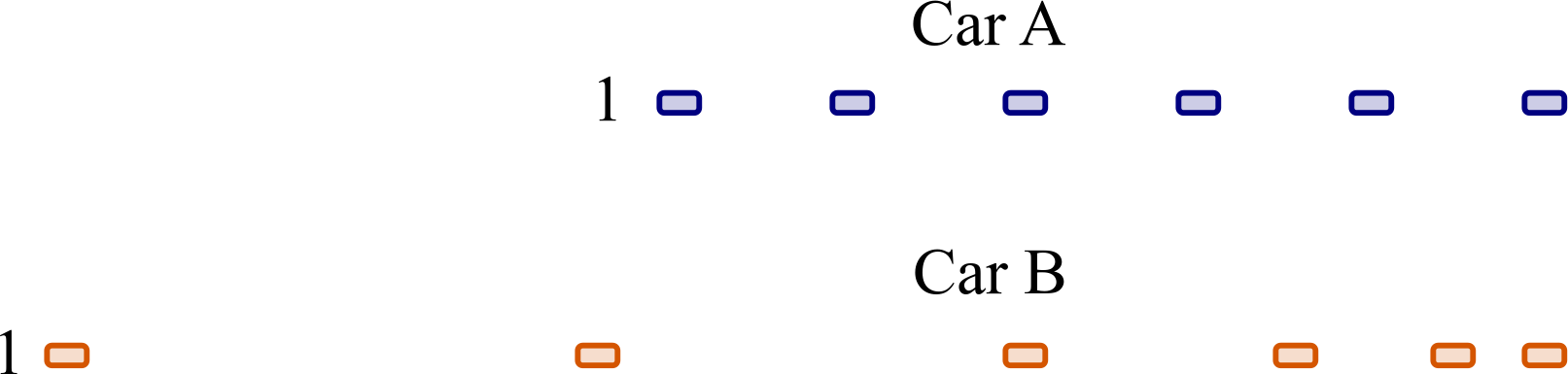
The simplest possible motion is motion along a straight-line path with a constant, unvarying speed. Let’s imagine a car that is driving to the right at a constant speed. Suppose you take images at a regular time interval, once every second:
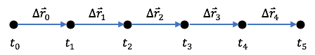
You can apply the particle model and represent the car as a point object, creating a motion diagram showing the position of the car at each instant of time and the corresponding displacement vectors.
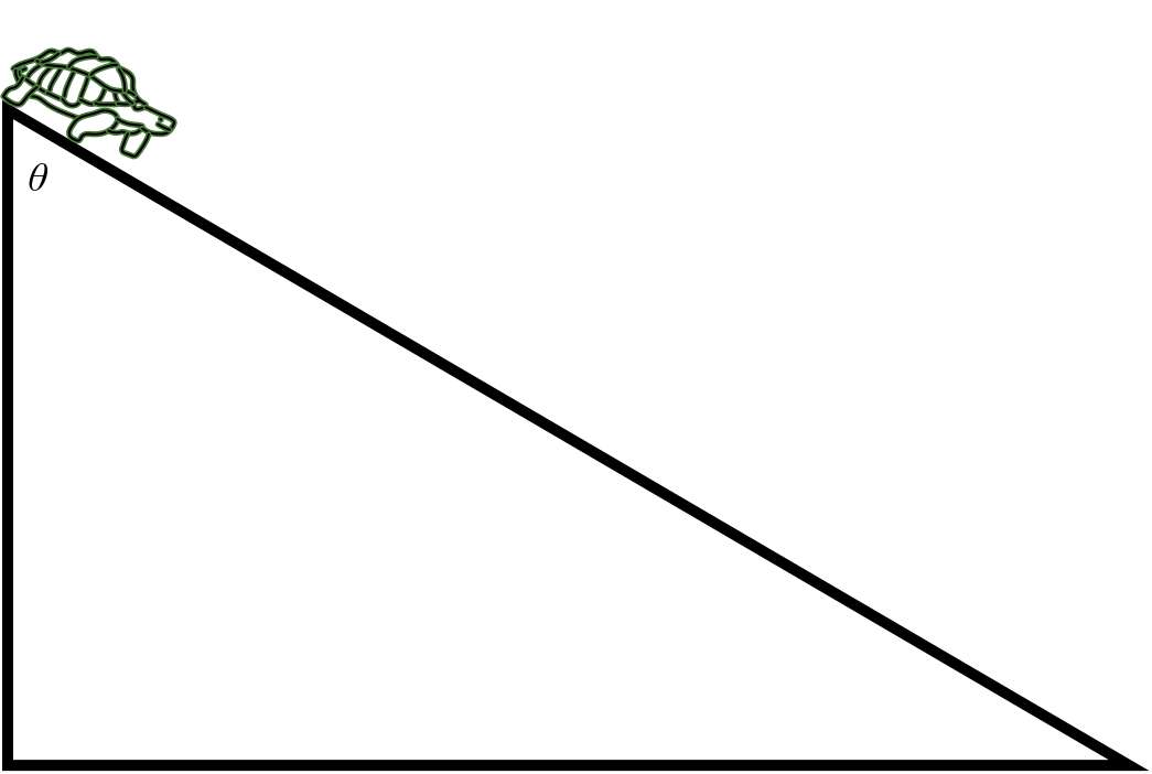
It takes \(40 \mathrm{~s}\) for a tortoise to travel down the slide shown in the figure below. Its initial speed is \(0 \mathrm{~m/s}\) and its final speed is \(0.2 \mathrm{~m/s}\) down the ramp. Assume the slide is \(4 \mathrm{~m}\) long and the given angle is equal to \(22^o\text{.}\)
Draw a right triangle where the hypotenuse is the average acceleration vector and the legs represent the horizontal and vertical components. Be sure to label the given angle \(\theta\) carefully in your triangle!
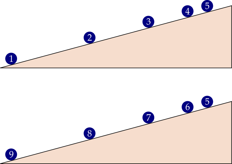
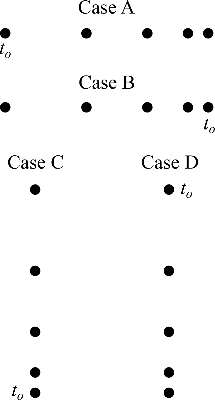
A total of \(0.2 \mathrm{~s}\) passes between each successive dot in the strobe diagram below. The distance between the leftmost and rightmost points is \(64 \mathrm{~cm}\text{.}\)
Sketch motion graphs for the ball showing position, velocity, and acceleration vs. time. Confirm that your graph agrees with the derivative relationships between position, velocity, and acceleration.
Why do you think working with so many different representations is useful in physics? Cite some specific activities where different representations have led you to understand something differently.
You and a friend are each riding a bicycle. You are moving \(8 \mathrm{~m/s}\) to the west relative to the ground. Your friend is moving \(12 \mathrm{~m/s}\) to the west relative to the ground.
The strobe diagram below shows a ball moving from left to right. A total of \(1 \mathrm{~s}\) has passed between each successive dot. The distance between the leftmost and rightmost points is \(12 \mathrm{~m}\text{.}\)
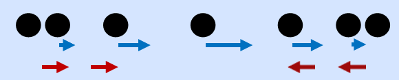
The instantaneous velocity vectors (middle, blue) can be found by looking at the change in position on either side of each dot. The average acceleration vectors (bottom, red) can be found by looking at the change in velocity at the start and end of each interval. This diagram assumes that the speed at the start and end is zero, and that the acceleration is zero during the middle.
The velocity always points to the right, and the speed is first increasing and then decreasing. This can be seen by using the definition of velocity, which is the change in position divided by the change in time.
The instantaneous speed is the magnitude of the change in position divided by the change in time. The change in time is the same for each successive instant in a strobe diagram, so you only have to look at the change in position. Given that the objects are draw farther apart in the middle, the change in position has a bigger magnitude there, and therefore the instantaneous speed is also greater!
You have a tennis ball that you throw directly upward with initial speed \(v\text{.}\) The ball rises to height \(h\text{,}\) then falls back down. At time \(t\text{,}\) you catch the ball when it is moving downward with the same speed \(v\text{.}\)
Calculate (1) the average velocity of the tennis ball during this time interval and (2) the change in velocity of the tennis ball over this time interval.