Section 25.1 Equipotential Graphs
Subsubsection Key Ideas
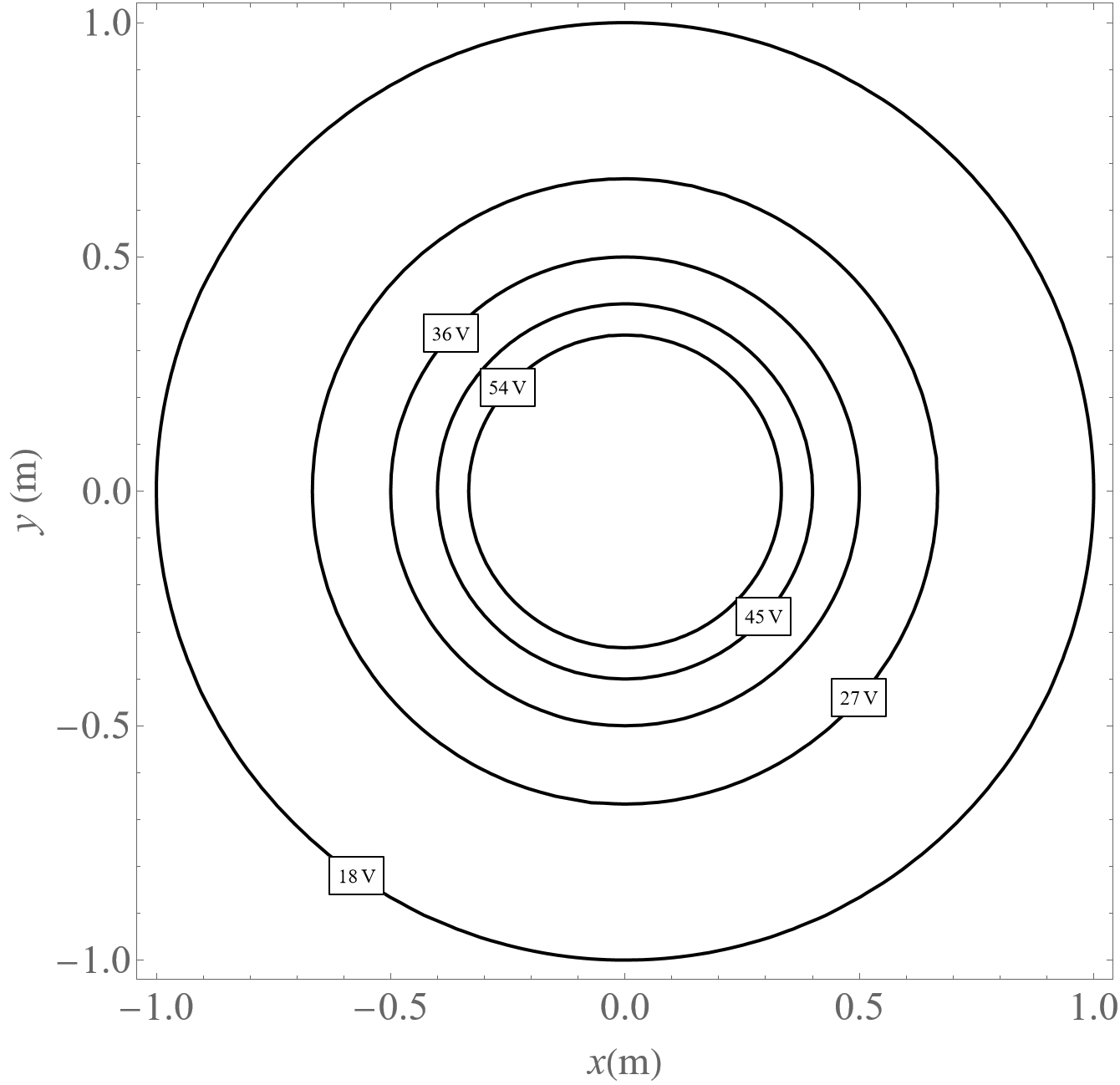
Similar to contour or topographical maps, equipotential graphs are extremely useful to see where the electric potential is constant throughout some region of space. Typically, equipotential lines will be drawn with the same difference in potential between two adjacent lines.
Representation 25.1.2. Equipotential Graphs.
An equipotential graph uses contour lines to show the electric potential.
-
The potential is constant along a line: Each line corresponds to a single value of the potential.
-
Adjacent lines are separated by the same voltage: The separation between adjacent lines can be any number of volts, but it must be the same for the entire graph.
-
Equipotentials are three-dimensional: The electric potential is a scalar field of all three spatial dimensions. Equipotential surfaces can be hard to draw, so it is common to represent cross-sections as equipotential lines in two dimensions.
-
The electric field points perpendicular to the equipotentials: The magnitude of the electric field can be estimated by looking at the local density of the equipotential lines.
Subsubsection Activities
Explanation 25.1.1. Moving through Equipotentials.
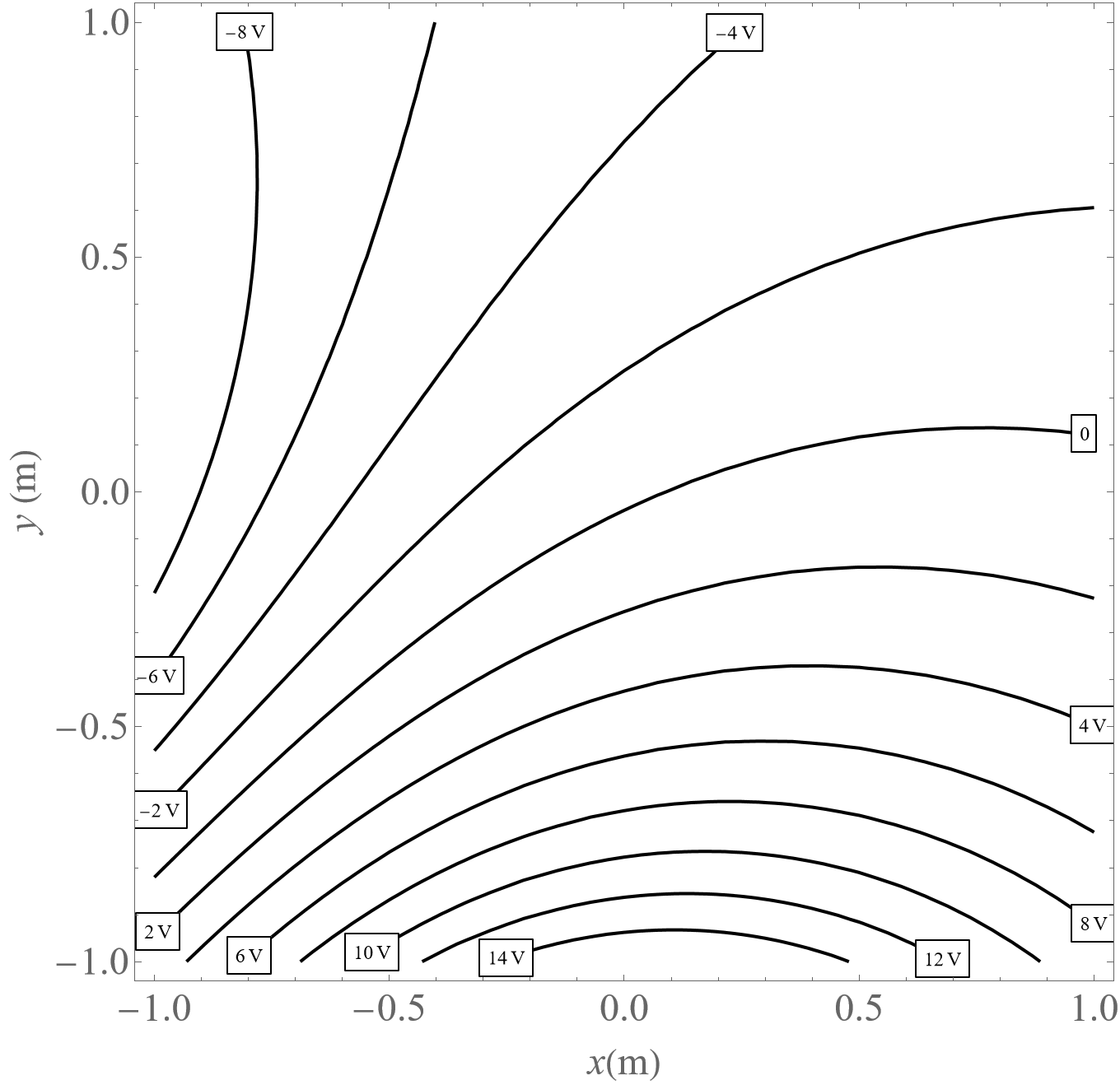
Consider the equipotential graph shown below.
(a)
Suppose you are initially located at \(x = 0\) and \(y = -1 \mathrm{~m}\text{.}\) Describe how the electric potential changes as you walk in the positive \(y\)-direction toward the top of the graph. Explain your reasoning.
(b)
Describe how the magnitude of the electric field \(|\vec{E}|\) changes as you walk in the positive \(y\)-direction toward the top of the graph. Explain your reasoning.

