Section 27.9 Ampère’s Law
Subsubsection Key Ideas
Definition 27.9.2. Ampère’s Law.
Ampère’s Law relates the magnetic field around a closed curve to the current passing through the region bounded by the curve:
\begin{equation*}
\oint_S \vec{B}\cdot d\vec{l} = \mu_0 I_{enclosed}
\end{equation*}
This is a line integral, like the integral for Determining the Electric Potential Difference from the Electric Field. The circle over the integral symbol indicates that this is an integral over a closed path: when this is true, the line integral is known as the circulation of the magnetic field.
Ampère’s Law (like Gauss’s Law) is extremely useful when your current distribution has just the right symmetry. To use Ampère’s Law effectively, you need:
-
the magnetic field to be parallel or perpendicular to the path \(d\vec{l}\)
-
the magnetic field to be uniform along the path
These conditions will simplify the dot product and the integral, allowing the magnitude of the magnetic field to be pulled out of the integral.
Subsubsection Example Derivation: Infinite Wire
A straightforward application of Ampère’s Law is to confirm that the magnetic field created by a very long wire carrying constant current \(I\) is
\begin{equation*}
\vec{B} = \frac{\mu_0}{2\pi}\frac{\vec{I} \times \hat{s}}{s}
\end{equation*}
The system exhibits cylindrical symmetry: that is, the magnetic field only depends on the distance \(s\) away from the axis where the wire lies, and it points only in the \(\hat{\phi}\) direction. As a result, a circle of radius \(s\) is a natural choice for the Amperian loop. The total current flowing through this loop is exactly \(I\text{,}\) so all that is left to calculate is the line integral:
\begin{equation*}
\oint_S \vec{B}\cdot d\vec{l} = \int_0^{2\pi} \left( B_\phi \hat{\phi} \right) \cdot \left( s d\phi \hat{\phi} \right) = B_\phi s \int_0^{2\pi}d\phi = 2\pi s B_\phi
\end{equation*}
Here \(B_\phi\) represents the magnitude of the magnetic field’s circumferential component (the component that points around the wire). The other components of the magnetic field are zero. Relating this to the current via Ampère’s Law results in the correct magnitude of the magnetic field!
\begin{equation*}
B_\phi = \frac{\mu_0 I}{2\pi s}
\end{equation*}
Subsubsection Activities
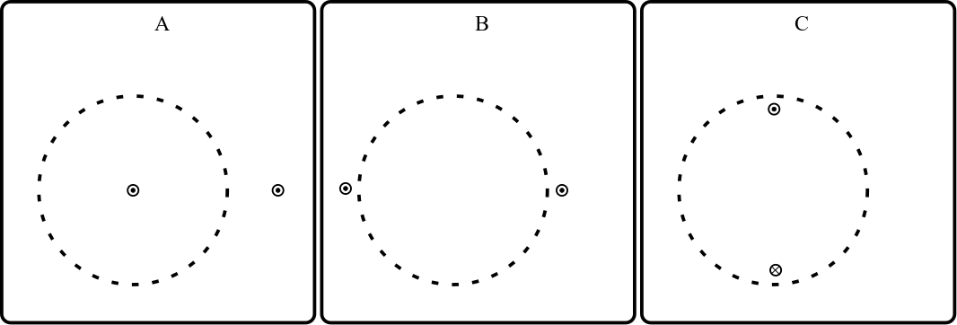
Explanation 27.9.1. Three Loops.
Shown below are three different cases, each with two identical current-carrying wires and a circular Amperian loop. In which case is the circulation of the magnetic field around the loop the largest?