The models you have built for simple harmonic motion have not included dissipative forces such as friction or drag. You know from experience that a pendulum left to oscillate will lose energy. The amplitude decreases in time until all energy has been dissipated and the system comes to rest. An oscillation whose amplitude decreases in time is called a damped oscillation.
The damping constant, \(b\text{,}\) depends on the shape of the object and the viscosity of the air (or other medium) in which it moves. The damping constant plays the same role as the coefficient of friction. The negative sign reminds you that the direction of the drag force always opposes the direction of the object’s velocity, as shown in the figure below.
Note that \(\omega_{d}\) is only valid when \(\frac{k}{m} \gt \frac{b^2}{4m^2}\text{.}\) 1
When this condition is met, the solution above is valid and the system is called “underdamped”. When this condition is not met, the solution will take on a different functional form.
This is the equation of motion for a damped mass on a spring. If you expect motion that is still oscillatory with an amplitude that decreases in time, you can guess a solution of the form:
\begin{equation}
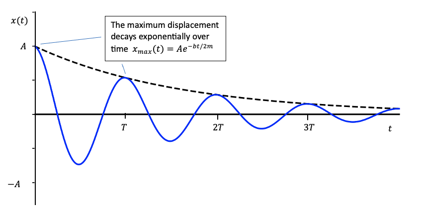
x(t) = x_{\text{max}} e^{-bt/2m} \cos{(\omega_{d} t +\phi_o)}\tag{16.11.2}
\end{equation}
This function turns out to satisfy the differential equation above, with an oscillation frequency given by:
Note that \(\omega_{d}\) is only valid when \(\frac{k}{m} \gt \frac{b^2}{4m^2}\text{.}\) When this condition is met, the solution above is valid and the system is called “underdamped”. When this condition is not met, the solution will take on a different functional form.
Sensemaking: A good sensemaking technique in situations like this is to plug the solution back into the equation of motion and confirm that \(x(t)\) is a solution!
You can see that the oscillation frequency is equivalent to the original oscillation frequency modified by the quantity \(b^2/4m^2 \text{.}\) In the Damped Spring Motion Graph the cosine function is modified by an exponential decay. You can see that the envelope of the amplitude decays in time. The maximum displacement away from equilibrium decreases according to the function
The damping constant characterizes the magnitude of the the drag force. Confirm that when \(b = 0\) you recover the position function and oscillation frequency for the un-damped mass on a spring.
This quantity has units of seconds, which suggests that it is a time of some kind! In fact, it is often known as the time constant, symbolized by \(\tau\text{.}\)
Use a graphing calculator (such as Desmos) to create a graph of \(x(t)\text{.}\) Choose starting values of the various constants such that you observe many oscillations (you likely want to choose a small value of \(b\)). Describe what the graph looks like in words.
For each of the following quantities, observe how the graph you made in the previous activity changes when you increase it and write a brief description of the change.